Introduction to Machine Learning and Neural Networks for Java Developers

If you are a typical software developer, all the machine learning buzz might seem confusing to you, especially when it comes to heavy math and statistics stuff that you haven’t been using for years or maybe never really understood.

This article aims to explain machine learning so you can have a better idea how you can use it and benefit from it. To achieve this, we’re going to reuse your existing Java knowledge and extend it with new machine learning concepts. After we cover the basics by exploring a Java code example for spam email classification using neural networks, everything else about how machine learning works should make more sense to you.

The example explored in this article uses Deep Netts, a Java-based deep learning development platform that provides a pure Java, open source, community edition of the Deep Netts deep learning engine. This engine is a reference implementation for the Visual Recognition (VisRec) API developed within the JCP as JSR 381, and it is a part of the efforts for standardizing APIs and evolving machine learning support for the Java platform.

One of the main ideas behind Deep Netts is to provide an intuitive and easy-to-use API that will enable Java developers to apply machine learning using their existing Java knowledge; simplify integration, deployment, and maintenance of machine learning solutions; and improve the overall developer experience.

What Is Machine Learning?

Machine learning is a type of computer algorithm that is able to adjust a set of its own internal parameters using sample data in order to perform a specific task on similar data.

Let’s take a more detailed look at this. Machine learning is an algorithm, pretty much like a sorting algorithm, which performs various operations with in-memory data structures. Usually this algorithm has a number of parameters that determine its operation. What makes it special is that it is able to adjust its own parameters using sample data, and this process is referred to as learning or training.

You can think of machine learning as a kind of self-configurable algorithm. A machine learning algorithm trained for specific data or a specific problem is called a model. Sample data used to train the model is called the training set.

Once a model is done with training, it can perform some specific task, for example, assign a category label to some input (classification) or estimate some quantity (regression). Both of these tasks are sometimes referred to as prediction. It’s also important to note that it’s expected that models will make mistakes (errors) in these predictions, and that these tasks will be performed with a certain degree of accuracy.

As long as appropriate data about the problem is available, machine learning can be useful for solving tasks that are difficult or impossible to solve directly using a fixed set of rules or formulas.

Example Use Case: Spam Classification

Email spam classification is a simple example of a problem suitable for machine learning. The task is to determine whether some email is spam or is not spam. As you probably know from personal experience, there are cases when this can’t be easily decided only by keywords in the subject or message, and additional properties of email message need to be taken into account. One way to solve this is to gather a set of example emails for spam and non-spam, and train a machine learning model.

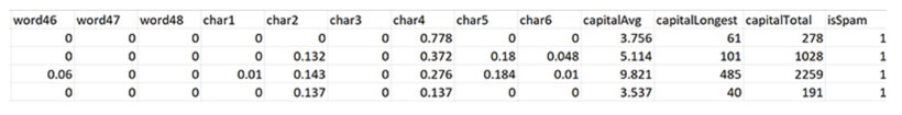
There is a publicly available data set that we’ll use, which contains 4,000 emails labeled in Figure 1 as spam (1) or non-spam (0). The data set is available as a CSV file, which is a commonly used format for machine learning data sets. For every email, there are 48 features that correspond to the frequency of occurrence of specific words; 6 features that correspond to the occurrence of specific characters, 3 features that correspond to the occurrence of capital letters; and the last feature, which corresponds to the spam/non-spam label. This type of task, in which you have to assign items to one of two categories, is called binary classification. Figure 1 shows a few sample lines from the CSV file.

In order to build a binary classifier for the given CSV file, we need to perform following steps:

1. Read data from the CSV file and create an in-memory data set.
2. Configure and create a neural network for binary classification tasks.
3. Train the neural network using the loaded data set.
4. Test the trained model to see how well it is performing.

Let’s get to the code. Listing 1 is a Java code snippet for creating a binary classifier using a feed-forward neural network for a given CSV file in just few lines of code. It is using the community edition of Deep Netts. Table 1 is an overview of the classes and methods used in Listing 1. Listing 1.

A few lines of code for building a binary classifier.

// Read data from a csv file and create data set
DataSet emailsDataSet= DataSets.readCsv(“spam_data_preprocessed.csv”, 57, 1, true); 

// create and configure an instance of feed forward neural network using builder
FeedForwardNetwork neuralNet = FeedForwardNetwork.builder()
                                             .addInputLayer(57)                          
                                                                                                                                                   
                                             .addFullyConnectedLayer(15) 

                                             .addOutputLayer(1, ActivationType.SIGMOID) 
                                                                             
                                             .lossFunction(LossType.CROSS_ENTROPY) 
                                             .build();

Table 1. Classes and methods used in Listing 1

The feed-forward neural network used in this example is a machine learning algorithm that is represented as a graph-like structure in Figure 2. Each node in this graph performs some calculation, which transforms its input. Each node applies some function to all of the inputs it receives from other nodes, and each node sends its result to the other nodes it is connected to. Nodes in this graph are organized into groups called layers. All nodes receive inputs from nodes in the previous layer and send output to nodes in the next layer. This results in a forward signal flow, and that’s where the name comes from.

There is very rough analogy between the kind of interaction shown in the computational graph and the way the neuron cells in a brain interact, and that’s why these graphs are also referred to as a neural network. Each connection between two nodes has an internal parameter called connection weight, and by adjusting these parameters during the training procedure, these graphs are configured to perform some desired behavior. The network learns by adjusting these parameters using a mathematical procedure to make the difference between the target outputs specified in a data set and the outputs of the network as small as possible. The difference between the target and network outputs is calculated using a so-called error function (aka a loss function).

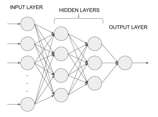
A feed-forward neural network must have only one input layer, only one output layer, and one or more hidden layers.

The input layer accepts external input (in this example, an email feature array), and the output layer provides the end result, which in our spam example is the probability that email is spam.

The number of nodes in the input layer corresponds to the number of input features in the data set, and the number of nodes in the output layer corresponds to the number of outputs in the data set. The size of the layers and the number of hidden layers are configurable parameters, and the optimal values depend on the problem and the data. In its simplest form, these parameters are determined experimentally, but there are also advanced algorithms to automatically search for optimal values for these parameters. In this type of neural network, hidden layers are so-called fully connected layers, which means that each node in a layer is connected to all the nodes in the previous layer.

In Listing 1, the feed-forward network has been configured to work as a binary classifier by setting functions that are commonly used for this type of task: ActivationType.RELU for the hidden layer, ActivationType .SIGMOID for the output layer, and LossType.CROSS_ENTROPY for the error function.

Listing 1 can be used as a template for other binary classification data sets. You just need to change the number of nodes in the input and output layers and tweak the hidden layers, as shown in Table 2. A feed-forward network can also be used for other types of machine learning tasks by setting the appropriate error and activation functions.

Table 2. Feed-forward network’s main configuration parameters.

How to Prepare the Data for Neural Network Training

In most cases, data from a CSV file needs to be prepared so it can be used for neural network training. In order for a neural network to be able to use data, the data needs to be transformed into numeric values (0 and 1) in a range. The data transformation operation that scales data to some range is called normalization. In the Deep Netts API, this operation is provided by the MaxNormalizer class.

The trained machine learning model will be used in production with some new (hopefully similar) data that has not been used for training. To estimate the classification accuracy on unseen data, the available data set is randomly split into a training set and a test set, which are then used for training and testing respectively. The ratio between the training and test set split is usually 60% for training and 40% for testing or 70% for training and 30% for testing, depending of the amount of available data. Example code for loading, preprocessing, and splitting data into training and test set is shown in Listing 2.

Listing 2. Normalizing and splitting data into training and test sets.

// Read data from csv file
DataSet emailsDataSet= DataSets.readCsv(“spam_data_preprocessed.csv”, 57, 1, true); 


// Split available data into training and test set at 60:40 ratio
DataSet[] trainAndTestSet = emailsDataSet.split(0.6, 0.4);


// Normalize data
MaxNormalizer norm = new MaxNormalizer(trainTestSet[0]); // create and initialize normalizer 
norm.normalize(trainTestSet[0]); // normalize training set
norm.normalize(trainTestSet[1]); // normalize test set

How to Train a Neural Network

After you have prepared the data and created the neural network, the next step is to train the neural network. A feed-forward neural network is trained using a backpropagation algorithm, which is a commonly used algorithm for various types of problems and neural networks. The Deep Netts API provides an implementation of this algorithm in the BackpropagationTrainer class. The method NeuralNetwork.getTrainer() returns an instance of the trainer that will be used to train the parent network. After setting a few parameters that control the algorithm’s behavior, the train method is invoked on a neural network using the training set as a method parameter, which starts the training procedure. This process is shown in Listing 3. Table 3 shows the backpropagation trainer configuration parameters, and Output 1 shows the total data set error and accuracy over training iterations (epochs).

Listing 3. Configuring and starting training.

      // configuring trainer
      neuralNet.getTrainer().setMaxError(0.03f)
                              .setMaxEpochs(10000)
                              .setLearningRate(0.001f);

      // start training using specified training set
      neuralNet.train(trainingSet);

Table 3. Backpropagation trainer configuration parameters.

Output 1. Total data set error and accuracy over training iterations (epochs)

TRAINING NEURAL NETWORK
-----------------------------------------------------------------------------------------------
Epoch:1, Time:72ms, TrainError:0.66057104, TrainErrorChange:0.66057104, TrainAccuracy: 0.6289855
Epoch:2, Time:18ms, TrainError:0.6435114, TrainErrorChange:-0.017059624, TrainAccuracy: 0.65072465
Epoch:3, Time:17ms, TrainError:0.6278175, TrainErrorChange:-0.015693903, TrainAccuracy: 0.6786232
Epoch:4, Time:14ms, TrainError:0.60796565, TrainErrorChange:-0.019851863, TrainAccuracy: 0.726087
Epoch:5, Time:15ms, TrainError:0.58832765, TrainErrorChange:-0.019638002, TrainAccuracy: 0.74746376
Epoch:6, Time:15ms, TrainError:0.5712807, TrainErrorChange:-0.017046928, TrainAccuracy: 0.7572464

How to Test a Classifier

In order to make sure that the trained classifier will provide an acceptable level of accuracy while classifying new emails, we’re going to perform a test procedure (aka an evaluation procedure). A test procedure for a classifier performs classification on test data that has not been used for training the classifier. It counts the correct and wrong classifications, and it calculates various additional metrics that help you understand various properties of the classifier. The Deep Netts API provides an easy way to perform a test procedure using just one call to a utility method from the Evaluators class (shown in Listing 4), which returns an object that contains a map of classification-specific metrics. Output 2 shows the most-important evaluation results that explain various classifier performance metrics.

Listing 4. Calling the utility method

EvaluationMetrics em = Evaluators.evaluateClassifier(neuralNet, testSet);
System.out.println(em);

Output 2. Evaluation results that explain various classifier performance metrics

Accuracy: 0.89402175 (How often is classifier correct in total)
Precision: 0.8658368 (How often is classifier correct when it gives positive prediction)
Recall: 0.8658368 (When it is actually positive class, how often does it give positive prediction)
F1Score: 0.8658368 (Average of precision and recall)

How to Use a Trained Classifier

Now that we have a trained classifier, we can use it to classify some new emails. Listing 5 shows example code:

Listing 5. Using the trained spam classifier

        // create binary classifier using trained network
        BinaryClassifier binClassifier = 
                                                new FeedForwardNetBinaryClassifier(neuralNet);        
        // get test email as an array of features
        float[] testEmail = testSet.get(0).getInput().getValues();

        // get probability score that email is spam
        Float result = binClassifier.classify(testEmail);
        System.out.println("Spam probability: "+result);  

The trained network is wrapped with the FeedForwardNetBinaryClassifier class, which makes it intuitive what the network does, how to use it, and what the inputs and outputs are. The BinaryClassifier interface from the Visual Recognition API uses generics to specify the type of inputs for a specific binary classifier, which in this case is an array of email features. Note that this can be relatively easily changed to some user-defined class.

An email to classify is provided from test set as an array of email features (the same set of features that we used to train the classifier). This array is then used as input for the classify method of the classifier.

The classification result for the binary classifier is given as a probability score, which indicates how likely it is that the given email is spam.

Code for the Complete Example

The full Java code for this spam classifier example, which includes loading, data preprocessing, training, and testing, is available as a Maven project on GitHub. Listing 6 shows the full workflow.

Listing 6. Full workflow for neural network based spam classifier

        
	    int numInputs = 57;
        int numOutputs = 1;
        
        // load spam data  set from CSV file
        DataSet emailsDataSet = 
                                    DataSets.readCsv(csvFile, numInputs, numOutputs, true);                   

        // split data set into train and test set
        DataSet[] trainAndTestSet = emailsDataSet.split(0.6, 0.4);
        DataSet trainingSet = trainAndTestSet[0];
        DataSet testSet = trainAndTestSet[1];
        
        // scale data to [0,1] range since this is the value range at which nn operates
        MaxNormalizer norm = new MaxNormalizer(trainTest[0]);
        norm.normalize(trainingSet);
        norm.normalize(testSet);
        
        // create instance of feed-forward neural network using its builder
        FeedForwardNetwork neuralNet = FeedForwardNetwork.builder()
                .addInputLayer(numInputs)
                .addFullyConnectedLayer(15)
                .addOutputLayer(numOutputs, ActivationType.SIGMOID)
                .lossFunction(LossType.CROSS_ENTROPY)
                .randomSeed(123)
                .build();

        // set training settings
        neuralNet.getTrainer().setMaxError(0.03f)
                              .setMaxEpochs(10000)
                              .setLearningRate(0.001f);
        
        // start training
        neuralNet.train(trainingSet);
        
        // test network and evaluate classifier
        EvaluationMetrics em = Evaluators.evaluateClassifier(neuralNet, testSet);
        System.out.println(em);
        
        // create binary classifier using trained network
        BinaryClassifier binClassifier = FeedForwardNetBinaryClassifier(neuralNet);        
        float[] testEmail = testSet.get(0).getInput().getValues();
        Float result = binClassifier.classify(testEmail);
        System.out.println("Spam probability for the given input: "+result); 
 

Learn More

To learn more about machine learning and deep learning, take a look at the series of blog posts on the Deep Netts blog. These posts describe in more detail how these algorithms work, other types of neural networks, and machine learning tasks.

• Machine Learning Tutorial for Java Developers
• From Basic Machine Learning to Deep Learning in 5 Minutes
• Deep Netts Community Edition on GitHub

About the Author

Zoran Sevarac is an associate professor at the University of Belgrade where he teaches Java and AI. He is a Java Champion, a JCP member, one of the JSR 381 expert group leads, a Duke’s Choice Award winner for project Neuroph, and a NetBeans contributor. His work at the moment is focused on making Java stronger and more developer friendly for machine learning.